Could be worse - Random topics in statistical physics, spin glasses, optimization and average case hardness

The Random Energy Model – Part I

28 December 2025 | E. Malatesta

Main definitions

The Random Energy Model (REM) is probably the easiest disordered system model with a non-trivial (spin glass) behaviour. It has been introduced and solved by B. Derrida (Derrida (1980)). It consists in having $2^N$ random independent energy levels $E_i$ each one being extracted from a Gaussian distribution, which I take for simplicity to be having zero mean and variance $N J$

$$\rho_N(E) = \frac{e^{-\frac{E^2}{2NJ}}}{\sqrt{2\pi N J}} \,.$$

In the following I will call by ''disorder'' the realization of the energy level samples.

Boltzmann-Gibbs distribution and thermodynamic quantities

Given an instance of the energy levels $\{E_i\}_{i=1}^{2^N}$ we assign to each of them a weight given by the Boltzmann-Gibbs distribution

$$\mu_{\beta}(E_i) = \frac{e^{- \beta E_i}}{Z_N(\beta)}$$

where $\beta = 1/T$ is the inverse temperature and the normalization constant $Z_N(\beta)$ is the so-called partition function

$$Z_N(\beta) = \sum_{i=1}^{2^N} e^{- \beta E_i} \,.$$

From the knowledge of $Z_N(\beta)$ we can compute the (intensive^[1]) free energy of the model

$$f_N(\beta) = - \frac{1}{\beta N} \ln Z_{N}(\beta)$$

The free energy in turn gives access to all thermodynamic quantities of interest. Denoting by $\langle \bullet \rangle$ the average with respect to the Boltzmann-Gibbs distribution (2) we can compute the energy

$$e_N(\beta) \equiv \frac{\langle E \rangle}{N} = \frac{1}{N Z_{N}(\beta)} \sum_{i=1}^{2^N} E_i \, e^{-\beta E_i} = \frac{\partial (\beta f_N(\beta))}{\partial \beta}$$

and the entropy by

$$s_N(\beta) = \beta (e_N(\beta) - f_N(\beta)) = \beta^2 \frac{\partial f_N(\beta)}{\partial \beta}$$

Large $N$ limit and self-averageness

Computing the partition function of the REM is not an easy task. Indeed, at variance with standard non-disordered models of statistical mechanics, the Boltzmann-Gibbs distribution $\mu_{\beta}(E_i)$, and therefore also $Z_N(\beta)$ and $f_N(\beta)$ are themselves random variables as they all depend on the realization of the $2^N$ energy levels.

Luckily, when we perform the thermodynamic limit $N\to \infty$, usually many simplifications arise, as the properties of intensive observables become independent of the disorder or the sample realization. In other words, the probability distribution of the free energy $f_N(\beta)$ becomes peaked around its expected value. Formally, for any $\epsilon>0$ it holds that

$$\lim_{N\to \infty} \mathrm{Pr} \left[ \left| f_N - \mathbb{E} f_N \right| > \epsilon \right] = 0$$

where I have denoted by $\mathbb{E}[\bullet]$ the average over disorder given in (1). An observable satisfying such property is called self-averaging in statistical physics; this is equivalent to the concept of concentration of a random variable in math. This means that $f_N$ does not appreciably fluctuate from sample to sample when $N$ is large.

We are interested in studying the properties of the Boltzmann-Gibbs distribution in the limit $N\to\infty$.

Solving the REM using the microcanonical ensemble

Instead of working out with the temperature fixed (i.e. in the canonical ensemble), it is much easier to solve the REM by fixing the energy $e$, which in statistical mechanics is the so-called microcanonical ensemble. In this ensemble one aims to compute the entropy at fixed energy $e$ which is given by

$$s_N(e) = \frac{1}{N} \ln \Omega_N(e)$$

where $\Omega_N(e)$ is the the number of configurations with energies in the interval $[N e, Ne+\Delta E]$. It can be written as

$$\Omega_N(e) = \sum_{i=1}^{2^N} n_i(e)$$

with

$$n_i(e) = \left\{ \begin{align*} &1 \,, & E_i \in \left[N e, N e +\Delta E\right] \\ &0 \,, & \mathrm{otherwise} \end{align*} \right.$$

Note that $s_N(e)$ is itself a random variable, being dependent on the particular realization of the energy levels.

Physical range of energies of the REM

Markov's inequality bounds the probability that the a non-negative random variable is strictly positive by its average value. In our case the random variable $\Omega_N(e)$ is also integer valued, so one finds

$$\mathrm{Pr}[\Omega_N(e) > 0] = \sum_{n>0} \mathrm{Pr}[\Omega_N(e) = n] \le \sum_{n\ge 0} n \, \mathrm{Pr}[\Omega_N(e) = n] = \mathbb{E}[\Omega_N(e)]$$

This is also called first moment bound. Note that $\Omega_N(e)$ is a Bernoulli random variable $\Omega_N(e) \sim B(2^N, p_N(e))$, where

$$p_N(e) = \int_{Ne}^{N e + \Delta E } dE \rho_N(E) \simeq \rho_N(Ne) \Delta E$$

having assumed a narrow window of energies $\Delta E$ that does not scale with $N$. The average of $\Omega_N(e)$ over the realization of the energy levels is therefore simple to compute and gives

$$\mathbb{E} [\Omega_N(e)] = 2^N p_N(e) \sim e^{N\left(\ln 2 - \frac{e^2}{2J}\right)}$$

This quantity goes exponentially to zero when $N\to \infty$ if $|e| > e_0$ with

$$e_0 = \sqrt{2J \ln 2} \,.$$

From Markov's inequality one finds therefore that the probability of finding energy levels with $|e| > e_0$ is exponentially small in $N$. For this reason from now on we will consider as the physical interval of energies to be^[2]

$$e \in [- e_0, e_0] \,.$$

In this range the average number of energy levels with energy $e$, is exponentially large in $N$.

Self averaging property of $\Omega_N(e)$

I want to now show that in the large $N$ limit $\Omega_N(e)$ concentrates around its average value. This can be shown by computing its variance:

$$\mathrm{Var}[\Omega_N(e)] = 2^N p_N(e) (1-p_N(e)) = \mathbb{E}[\Omega_N(e)] - O(e^{-N})$$

where in the last step I have neglected exponentially small corrections in $N$. A simple application of Chebyshev's inequality gives $\forall \epsilon>0$

$$\mathrm{Pr}\left[\left| \frac{\Omega_N(e)}{\mathbb{E} [\Omega_N(e)]} - 1 \right| \ge \epsilon \right] \le \frac{\mathrm{Var}[\Omega_N(e)]}{\epsilon^2 \, \mathbb{E}[\Omega_N(e)]^2} \le \frac{1}{\epsilon^2 \, \mathbb{E}[\Omega_N(e)]} \overset{N\to \infty}{\longrightarrow} 0$$

that the random variable $\Omega_N(e)$ converges in probability exponentially fast in $N$ to its expected value.

This implies that average microcanonical entropy is given by

$$s(e) = \lim_{N\to \infty} s_N(e) = \lim_{N\to \infty} \frac{1}{N} \ln \mathbb{E} [\Omega_N(e)] = \left\{ \begin{align*} &\ln 2 - \frac{e^2}{2 J}\,, & |e| \le e_0 \\ & 0\,, & |e| > e_0 \end{align*} \right.$$

Note that this expression does not depend on the coarse-graining of the energy $\Delta E$.

The free energy

Having found the microcanonical entropy, I now wish to find the free energy of the model which requires the inverse temperature $\beta$ to be fixed. This can be obtained by the so called Legendre transform which is the way one passes from one ensemble to another in statistical mechanics. For the reader not familiar with changes of ensemble this is actually obtained by grouping configurations by their energy density $e$ and then integrating over all possible (allowed) energies $e$. Sending the coarse-graining $\Delta E$ to zero (after the limit $N\to \infty$) one finds

$$Z_N(\beta) = \sum_{i=1}^{2^N} e^{- \beta N e_i} = \int d e \, \sum_{i=1}^{2^N} \delta(e-e_i) e^{- \beta N e} = \int_{-e_0}^{e_0} d e \, e^{N (s(e) - \beta e)} \,.$$

For large $N$ the integral is dominated by the maximum of the argument of the exponential (Laplace's method), that is

$$f(\beta) \equiv \lim_{N\to\infty} f_N(\beta) = -\frac{1}{\beta} \, \max_{e \in [-e_0, e_0]} \left[s(e) - \beta e\right] \,.$$

The maximization imposes

$$\left. \frac{d s(e)}{d e}\right|_{e_\star} = - \frac{e_\star}{J} = \beta \; ⟹ \; e_\star = - \beta J \,.$$

This is valid only if $e_\star$ lies in the interval of allowed energy densities $[-e_0, e_0]$. The corresponding free energy being

$$f(\beta) = -\frac{1}{\beta} \left( \ln 2 - \frac{\beta^2 J}{2} + \beta^2 J\right) = -\frac{\ln 2 }{\beta} - \frac{\beta J}{2}$$

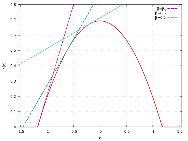
If $\beta$ is too large (i.e. the temperature too low), the maximum of (20) is given by $e_\star = -e_0$. This holds when

$$\beta \ge \beta_c \equiv \frac{e_0}{J} = \sqrt{\frac{2 \ln 2}{J}} \,.$$

In this regime the free energy is constant. Summarizing the free energy of the REM is

$$f(\beta) = \lim_{N\to\infty} f_N(\beta) = \begin{cases} -\frac{\ln 2 }{\beta} - \frac{\beta J}{2} & \; \mathrm{if} \;\beta< \beta_c \\ - \sqrt{2 J \ln 2} & \; \mathrm{if} \; \beta \ge \beta_c \,. \end{cases}$$

This shows that at $\beta = \beta_c$ the model exhibits a second order phase transition as the derivative of $f(\beta)$ is continuous at $\beta = \beta_c$, but its second order is not. This phase transition has different names in the literature: ''freezing'', ''condensation'' and ''random first order'' (RFOT) phase transition. The first two names refers to the fact that the system ''freezes'' or ''condenses'' into the states having lowest available energies, i.e. $E_i \simeq - e_0 N$.

The last name refers to the fact that while the transition is of second order in the classical sense, it discontinuous in terms of the order parameter. We have not introduced the order parameter in the REM model, but we will probably analyze it in a later post. Here I only anticipate the fact that at $\beta = \beta_c$ the Boltzmann-Gibbs measure in eq. (2) starts being dominated by subexponential number of configurations. This can be indeed verified by computing the entropy of the REM as a function of the temperature

$$s(\beta) = \beta^2 \frac{\partial f}{\partial \beta} = \begin{cases} \ln 2 - \frac{\beta^2 J}{2} & \; \mathrm{if} \;\beta< \beta_c \\ 0 & \; \mathrm{if} \; \beta \ge \beta_c \,. \end{cases}$$

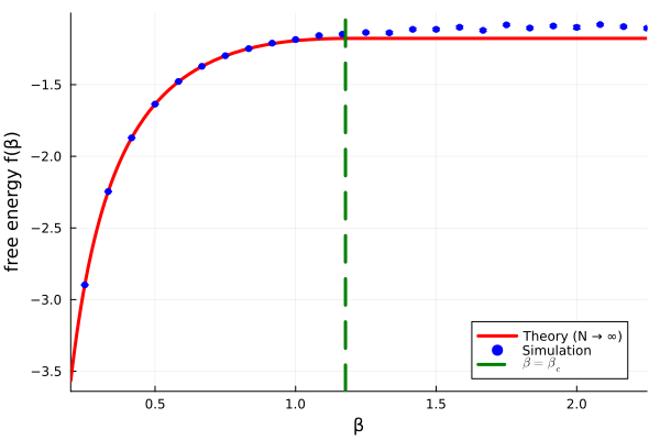
Numerical checks

Below I show a simple code that computes numerically the quenched average of the free energy of the REM by sampling independent Gaussian energy levels (with $J=1$).

using Random, Statistics, Plots, LaTeXStrings

"""
    Robust implementation of logsumexp
"""
logsumexp(x) = (m = maximum(x); m + log(sum(exp.(x .- m))))

"""
    One-sample REM free energy
"""
function rem_free_energy_sample(N::Int, β::Float64)
    M = 1 << N
    σ = sqrt(N)
    E = σ .* randn(M)
    logZ = logsumexp(- β .* E)
    return - logZ / (β * N)
end


"""
    Averaged REM free energy in the limit N → ∞
"""
function rem_free_energy_theory(β::Float64)
    βc = √(2log(2))
    if β <= βc
        return - log(2) / β - β / 2
    else
        return - √(2log(2))
    end
end

"""
    Computes the average over `nsamples` of the REM free energy
    for the values of β contained in the vector `βs`
"""
function simulate_curve(N::Int, βs::Vector{Float64}; nsamples::Int=30, seed::Int=23)
    if seed > 0
        Random.seed!(seed);
    end
    means = Float64[]
    stderrs = Float64[]
    for β in βs
        vals = [rem_free_energy_sample(N, β) for _ in 1:nsamples]
        push!(means, mean(vals))
        push!(stderrs, std(vals) / √nsamples)
    end
    return means, stderrs
end

"""
    Generates a plot comparing theory vs simulations
"""
function plot_rem_free_energy(; N=18, βmin = 0.25, βmax = 2.25, nβ=25,
                              nsamples=30,
                              seed=-23,
                              outfile="rem_free_energy.png")
    βc = √(2log(2))
    βs = collect(range(βmin, βmax, length=nβ))

    f_sim, f_err = simulate_curve(N, βs; nsamples=nsamples, seed=seed)

    plot(rem_free_energy_theory, xlim=(βmin-0.05, βmax);
        label="Theory (N → ∞)",
        linewidth=3, color=:red,
        xlabel="β", ylabel="free energy f(β)",
    )

    scatter!(βs, f_sim;
        yerror=f_err, color=:blue, markerstrokecolor=:blue,
        label="Simulation",
        markersize=3.5
    )

    vline!([βc]; label=L"\beta=\beta_c", linestyle=:dash, linewidth=3, color=:green)

    savefig(outfile)
end

plot_rem_free_energy(N=18, nsamples=30, outfile="./_assets/images/blog/rem_free_energy.png")

The results are summarized in the figure below. The numerical results reproduce the exact $N\to \infty$ free-energy curve and its freezing transition at $\beta=\sqrt{2 J \ln 2}$.

[1]	i.e. scaled with $1/N$.

[2]

Note that the value of the energy $e_0$ can be obtained by asking: given $M$ normal Gaussian variables $X$ with mean zero and variance $J=1$, what is the typical value attained by the maximum among those? This can be obtained by imposing that the probability of observing the random variable $X$ to be large than a (large) value $x_M$ is comparable to $1/M$ $$\mathrm{Pr}[X \ge x_M] = \int_{x_M}^{\infty} dy \frac{e^{-y^2/2}}{\sqrt{2\pi}} = \frac{1}{2} \mathrm{Erfc}\left( \frac{x_M}{\sqrt{2}}\right) \simeq \frac{e^{-x_M^2/2}}{\sqrt{2\pi} x_M} = \frac{1}{M}\,.$$ Taking logs one finds at the leading order in $M$ $$x_M ≃ \sqrt{2 \ln M} \,.$$ Using $M = 2^N$ and rescaling with $N$ one gets the result. By symmetry and a similar argument one also can get the value $-e_0$ by studying the minimum instead of the maximum.

References

[1] Derrida, Bernard, "Random-energy model: Limit of a family of disordered models", Physical Review Letters 45.2 (1980): 79.