Could be worse - Random topics in statistical physics, spin glasses, optimization and average case hardness
Chaos in Random Neural Networks
9 August 2026 | E. Malatesta
I recently went back to the classic paper of Sompolinsky, Crisanti and Sommers on chaos in random neural networks [Sompolinsky, Crisanti and Sommers (1988)], which was revisited in detail in [Crisanti and Sompolinsky (2018)].
The model they considered is a recurrent neural network with random asymmetric couplings. Its remarkable feature is that, using Dynamical Mean Field Theory (DMFT), one can show that in the large- limit the collective dynamics reduces to an effective one-neuron stochastic problem. The noise in this effective problem is generated self-consistently by the activity of the rest of the network.
In this first post I want to derive this reduction and the resulting closed equation for the autocorrelation function. I will then show how, in this model, the effective one-neuron problem can be recast as Newton's equation for a fictitious particle moving in a self-consistent potential. This mechanical analogy gives a very transparent way of organizing the formal DMFT solutions: static solutions, periodic solutions, and the special decaying solution associated with the chaotic phase.
The model
Consider continuous variables , representing the post-synaptic potentials of neurons. The activity, or output, of neuron is
Here is the gain and is an odd sigmoidal-shaped function. I will mostly keep the notation general, but the canonical example I will consider is . The dynamics of the post-synaptic potentials are given by the following coupled differential equations
The first term is the leak: without any input, decays exponentially to zero. The second term is the recurrent input from the rest of the network, which depends on the coupling matrix . Here we will consider random, independent, asymmetric couplings, having mean 0 and variance 1:
We also set , which is irrelevant at large . The scaling in equation (2) maintains each recurrent input of order one as .
The configuration where all the neurons are silent
is always a fixed point. Linearizing around it gives
Since the eigenvalues of fill the unit disk in the complex plane at large , the rightmost real part of the spectrum of is . Hence the zero fixed point is linearly stable for and loses stability at . This simple calculation identifies the transition point, but it does not tell us what happens for . For that we need the nonlinear mean-field theory.
Dynamical Mean Field Theory
Define the recurrent input to neuron :
The equation of motion becomes
The idea of dynamical mean-field theory (DMFT) is that, at large , becomes a Gaussian process. In the following we will perform a simple, naive computation, which gives the right equations.
At fixed trajectories , is a sum of many independent random variables. Its mean and covariance are:
At large , the empirical average appearing in the covariance self-averages and converges to a deterministic two-time autocorrelation function . The original -dimensional network can therefore be reduced to a single effective neuron driven by a Gaussian input with covariance
Here and in the following, denotes the average over the effective Gaussian process. The dynamics of the effective neuron is therefore
The covariance of the effective noise must be determined self-consistently from the activity of the effective neuron via
Thus, the original dynamics of the dimensional network has been replaced by a by a stochastic single-neuron problem whose noise statistics are generated self-consistently by the neuron itself. This is the central dynamical mean-field equation.
A small subtlety is hidden in this argument. The trajectories are generated by the same coupling matrix , so the factors cannot literally be regarded as fixed independently of the couplings . The reason the conclusion is nevertheless correct is the full asymmetry and mean-field scaling of the couplings and can be understood with a cavity argument, see the footnote[1]. The same result can be derived more systematically using the Martin–Siggia–Rose–Janssen–De Dominicis (MSRJD) generating-functional formalism; see [Crisanti and Sompolinsky (2018)]. For a pedagogical introduction to this method in the context of mean-field spin-glass dynamics, see [Castellani and Cavagna (2005)].
The autocorrelation equation
We now focus on a stationary state where two-time quantities like the activity autocorrelation depend only on the time difference
Similarly the post-synaptic field autocorrelation
Next, let's take the effective equation , multiply the left and the right hand side by and take the average with respect to :
The right and left hand side contain by definition respectively and . Using the fact that and one finds that the first order derivative cancel, obtaining
This is yet not enough, as we need to express self-consistently in terms of . The key simplification is that is Gaussian. Indeed since the effective equation (10) is linear in the solution can be written as
This is a linear functional of a Gaussian process, hence it is itself a Gaussian process. Therefore the pair on which depends is a two-dimensional Gaussian vector. Its covariance matrix is
A two-dimensional Gaussian is completely fixed by this covariance matrix. Therefore is a function of and :
We can represent the two correlated Gaussian variables using three independent standard Gaussians :
Then
So we find, using the fact that is an odd function
where we have introduced the notation . The closed DMFT equation is therefore
The unknown is a single function , and all dependence on the nonlinear transfer function is hidden in the scalar function .
Properties of
The equation (15) can be inverted explicitly, using the face that the Green function of the operator is
as . Therefore we find
This formula is useful because it gives the properties of directly. First, is an even function (the same is of course true for ). Secondly, is differentiable function with zero derivative in the origin[2]
Third, since is an autocorrelation, it obeys the Cauchy-Schwarz bound
Thus acceptable solutions must satisfy
Collecting everything, the steady-state DMFT solutions are curves satisfying
The initial condition must be chosen so that the resulting solution is self-consistent.
The Newtonian particle analogy
Much insight can be gained into the problem by rewriting the DMFT equation (22) as
where we have defined the potential[3]
The DMFT equation therefore turns out to be a Newton's equation for a particle with position , moving in the time variable , in the potential starting at position with zero velocity. The energy
is conserved. The important point is that the potential itself depends on . By changing we are not only changing the initial point of the Newtonian particle; we are also changing the shape of the potential in which it moves. We will see how the potential changes very concretely in the next section.
Therefore the problem is self-consistent in a very concrete mechanical sense. We must choose a starting point , build the potential , release the particle from rest at , and then check whether the orbit is an admissible autocorrelation.
The shape of the potential
In order to classify the possible solutions to the DMFT equation (29), it is useful to understand how the potential can look like vs , for each chosen initial condition .
Start noticing that for an odd transfer function, such as , the function is odd in . Therefore the potential in (30) is an even function of . Hence it is enough to study its shape when .
In the next discussion we will argue that the potential cannot have an arbitrary shape. We can see this by computing the first three derivatives of the potential. Using the fact illustrated in the footnote[3], it is easy to show that, for
Therefore is a monotonically increasing function of for . This is a rather strong constraint: the curvature can change sign at most once. As a consequence the potential can only have few qualitative shapes. We can distinguish between them by looking at the sign of the curvature of the potential at the origin. The first possibility is
Since the curvature is increasing for , the potential is convex. Because is even, is then the unique minimum. The potential is a single well. The second possibility is
Then is a local maximum. Since the curvature can change sign at most once, the potential can bend upward at only once in the physical interval . If crosses zero before the endpoint , this crossing gives a unique minimum at positive , and by evenness another minimum at negative . In that case the potential has the shape of a double well.
If does not cross zero before the endpoint , then we have a downhill potential as it is monotonically decreasing in the whole interval . As shown in the footnote[4] this case only happens when , which implies that in this regime the DMFT equation admits only the solution .
Thus the monotonicity of tells us that only very simple shapes are possible: a single well centered at the origin, a double well, or a downhill potential on the admissible interval.
The boundary between the single-well and double-well shapes given by the condition
In the case of the function, for small , the integral is close to one, so if the curvature at the origin is positive and the potential is a single well. As increases, the Gaussian variable explores the saturated part of , where is small. The integral decreases, the curvature at the origin eventually becomes negative, and the potential turns into a double well.
Static solutions
The simplest possible solution of the DMFT equation corresponds to an autocorrelation function independent of time
This corresponds to the particle not moving and sitting at the stationary points of the potential. This gives the condition
For , is always a solution. This is the silent fixed point of the original network. The argument of the previous subsection show in the footnote[4] shows that for this is the only admissible stationary DMFT solution. For equation (39) has also a nonzero solution .
Time-dependent solutions
We here analyze other solutions of the DMFT equation (29) for which are time-dependent. Since the motion conserves energy, at each time the energy stays equal to the initial one corresponding to the one of the particle being at rest at
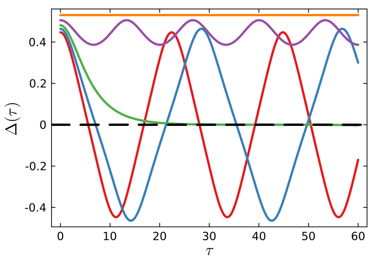
Different shapes of the potential lead to different types of formal DMFT solutions. If the initial condition is such that then the autocorrelation diplays an oscillatory, periodic profile. This corresponds to a limit cycle in the original network. Moreover if , then the changes sign (when the particle reaches ). If instead , then the particle is confined into the positive well of the potential, and the oscillations do not change sign.
There is also a special solution that separates those two regimes when
This solution decays to zero when for large
This suggests that the underlying neural dynamics is chaotic, as the networks tends to forget the initial condition.
Numerical illustration
We can clarify the previous classificationn of DMFT solutions, by simply solving (29) numerically for each given initial condition and showing the corresponding potential .
module SCS

using OrdinaryDiffEq, QuadGK, Roots

# ------------------------------------------------------------
# Gaussian integration
# ------------------------------------------------------------

const ∞ = 20.0
const dx = 0.5
const interval = map(x->sign(x)*abs(x)^2, -1:dx:1) .* ∞

G(x) = exp(-x^2/2) / √(2π)

∫D(f, int=interval) = quadgk(z->begin
        r = G(z) .* f(z)
        isfinite(r) ? r : 0.0
    end, int..., atol=1e-5, maxevals=10^5)[1]

# ------------------------------------------------------------
# Transfer function, its derivative and primitive
# ------------------------------------------------------------

ϕ(x) = tanh(x)
∂ϕ(x) = 1 - tanh(x)^2
Φ(x) = abs(x) + log1p(exp(-2abs(x))) - log(2) # Stable version of log(cosh(x))

# ------------------------------------------------------------
# F(Δ; Δ0)
# ------------------------------------------------------------

function F(Δ, Δ0, g)
    abs(Δ) < 1e-12 && return 0.0

    if Δ == Δ0
         return ∫D(z -> ϕ(g * √Δ0 * z)^2)
    end

    A = min(abs(Δ), Δ0)
    a = √(max(Δ0 - A, 0.0))
    b = √A

    m(z) = ∫D(x -> ϕ(g * (a * x + b * z)))

    return sign(Δ) * ∫D(z -> m(z)^2)
end

# ------------------------------------------------------------
# Potential V(Δ; Δ0)
# ------------------------------------------------------------

function V(Δ, Δ0, g)

    m1 = ∫D(x -> Φ(g * √Δ0 * x))

    if Δ == Δ0
        m1 = ∫D(z -> Φ(g * √Δ0 * z))
        m2 = ∫D(z -> Φ(g * √Δ0 * z)^2)

        return -0.5 * Δ0^2 + (m2 - m1^2) / g^2
    end

    A = min(abs(Δ), Δ0)
    a = √max(Δ0 - A, 0.0)
    b = √A

    m(z) = ∫D(x -> Φ(g * (a * x + b * z)))

    return - 0.5 * Δ^2 + (∫D(z -> m(z)^2) - m1^2) / g^2
end

# Curvature of the potential at the origin
function Vcurv0(Δ0, g)
    m = ∫D(x -> ∂ϕ(g * √Δ0 * x))
    return g^2 * m^2 - 1
end

# ------------------------------------------------------------
# The three phase-diagram curves
# ------------------------------------------------------------

# Boundary between single-well and double-well potential
function Δ0_boundary(g; Δmin = 1e-9, Δmax = 1.2)
    g < 1 && return NaN

    return find_zero(Δ0 -> Vcurv0(Δ0, g), (Δmin, Δmax), Bisection())
end

# Decaying solution: selects the initial condition such that Δ(τ) → 0 as τ → ∞
function Δ0_decay(g; Δmin = 1e-9, Δmax = 1.2)
    g < 1 && return NaN

    return find_zero(Δ0 -> V(Δ0, Δ0, g), (Δmin, Δmax), Bisection())
end

# Static, fixed point solution
function Δ0_static(g; Δmin=1e-9, Δmax = 1.2)
    g < 1 && return NaN

    return find_zero(Δ0 -> F(Δ0, Δ0, g) - Δ0, (Δmin, Δmax), Bisection())
end

# ------------------------------------------------------------
# Numerical solution of Newton's equation:
#
# Δ'' = Δ - F(Δ; Δ0)
# ------------------------------------------------------------

function rhs!(du, u, p, t)
    Δ, v = u
    Δ0, g = p

    du[1] = v
    du[2] = Δ - F(Δ, Δ0, g)
end

function orbit(Δ0, g; T = 60.0, dt = 0.05)
    init_cond = [Δ0, 0.0]
    tspan = (0.0, T)
    params = (Δ0, g)
    prob = ODEProblem(rhs!, init_cond, tspan, params)
    return solve(prob, Tsit5(); saveat = dt, abstol = 1e-8, reltol = 1e-8)
end


end
We recap here also the three special values of given by the conditions:
The first equation defines boundary between the single-well and double-well shapes; the second one selects the decaying solution for and finally the third one gives the static solution. Those three conditions are implemented respectively in the functions Δ0_boundary, Δ0_decay and Δ0_static in the julia code above.
In Figure 1 we show an example of the shapes of the potential for for several values of . In Figure 2 I show the corresponding trajectories . The script below was used to produce those two figures.
using Plots, Plots.PlotMeasures, LaTeXStrings, Printf
# ------------------------------------------------------------
# Example: g = 2
# ------------------------------------------------------------

g = 2

Δ_boundary = SCS.Δ0_boundary(g)
Δ_decay = SCS.Δ0_decay(g)
Δ_static = SCS.Δ0_static(g)

Δ0s = [Δ_boundary, (Δ_boundary+Δ_decay)/2, Δ_decay, (Δ_decay + Δ_static)/2, Δ_static]

# ------------------------------------------------------------
# Plot potentials
# ------------------------------------------------------------

pV = plot(xlabel = L"\Delta", ylabel = L"V(\Delta;\Delta_0)", legend = (0.45, 0.3), palette = :Set1)

for Δ0 in Δ0s
    Ds = range(-Δ0, Δ0; length = 400)
    lab = latexstring(@sprintf("\\;\\Delta_0=%.3f", Δ0))
    plot!(pV, Ds, [SCS.V(D, Δ0, g) for D in Ds], label = lab)
    scatter!(pV, [Δ0], [SCS.V(Δ0, Δ0, g)], label = false,  primary = false, markersize = 3)
end


hline!(pV, [0.0], color = :black, linestyle = :dash, label = false)

display(pV)


# ------------------------------------------------------------
# Plot Δ(τ)
# ------------------------------------------------------------

Δ0s = [Δ_boundary, (Δ_boundary+Δ_decay)/2, Δ_decay, (Δ_decay + Δ_static)/2, Δ_static]

pD = plot(xlabel = L"\tau", ylabel = L"\Delta(\tau)", legend = false, palette = :Set1)


for Δ0 in Δ0s
    sol = SCS.orbit(Δ0, g; T = 60.0, dt = 0.05)
    plot!(pD, sol.t, [u[1] for u in sol.u])
end

hline!(pD, [0.0], color = :black, linestyle = :dash)

display(pD)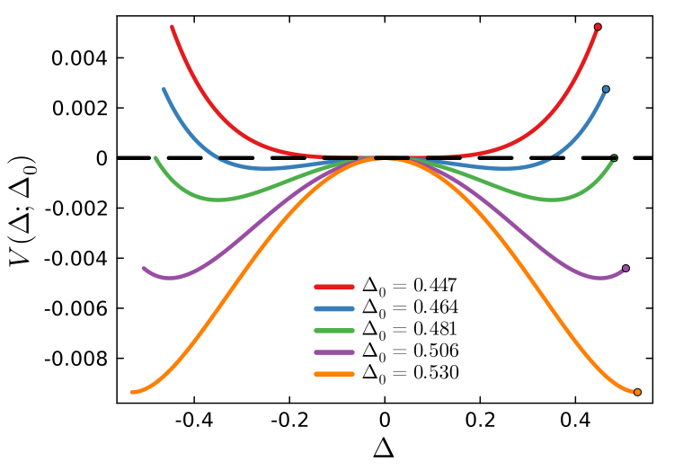
Phase Diagram
Finally we can compute the three boundaries given in (43), (44) and (45) for different values of and draw a phase diagram in the plane. This is done in the julia script below, and Figure 3 summarizes the result. Notice that all three curves meet at the transition point , .
# ------------------------------------------------------------
# Plot phase diagram
# ------------------------------------------------------------

gs = range(1.001, 100.0; length = 500)

Δ_boundary_curve = Float64[]
Δ_decay_curve = Float64[]
Δ_static_curve = Float64[]

for gval in gs
    push!(Δ_boundary_curve, SCS.Δ0_boundary(gval; Δmin = 1e-8, Δmax = 1.2))
    push!(Δ_decay_curve,   SCS.Δ0_decay(gval;   Δmin = 1e-8, Δmax = 1.2))
    push!(Δ_static_curve,  SCS.Δ0_static(gval;  Δmin = 1e-8, Δmax = 1.2))
end

push!(Δ_boundary_curve, 2/π)
push!(Δ_decay_curve,   2*(1-2/π))
push!(Δ_static_curve,  1.0)
gs = push!(collect(gs), Inf)


plt = plot(xlabel = L"\Delta_0", ylabel = L"1/g", legend = :topright, xlims = (0.0, 1.05), ylims = (0.0, 1.1)  )

plot!(plt, Δ_boundary_curve, 1.0 ./ gs, label = L"\;V''(0;\Delta_0)=0")
plot!(plt, Δ_decay_curve, 1.0 ./ gs, label = L"\;V(\Delta_0;\Delta_0)=0")
plot!(plt, Δ_static_curve, 1.0 ./ gs, label = L"\;F(\Delta_0;\Delta_0)=\Delta_0")

display(plt)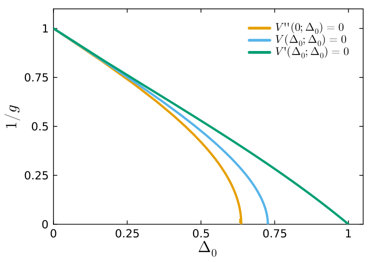
What's next?
I will deliberately leave two questions for a second post. First, for , the one-replica DMFT equation admits several formal solutions, and one has to understand which of them corresponds to a stable attractor of the original neural network dynamics. We will find out that the only physical DMFT solution is the decaying one. Secondly, one can ask whether this solution is genuinely chaotic. This leads naturally to the computation of the Lyapunov exponent.
| [1] | Remove neuron and denote by the trajectories of the remaining network. These cavity trajectories are independent of the couplings entering the removed neuron. Consequently, is, at large , a Gaussian process with covariance . Adding neuron back perturbs each of the other trajectories only by . Adding neuron back perturbs neuron through the connection . To first order in this perturbation, where measures the response of neuron at time to a perturbation at time . Each individual perturbation is therefore of order . Substituting this into the input to neuron , , gives The resulting correction to the input of neuron involves products . For fully asymmetric couplings, and are independent and centered, so these feedback contributions add incoherently and vanish in the large limit. Hence the true input and the cavity input coincide to leading order as . If reciprocal couplings were correlated, this cancellation would not occur and an additional retarded self-interaction term would survive in the effective dynamics. |
| [2] | Differentiating (24) gives At , using the evenness of , the two integrals are equal. |
| [3] | Note that i.e. the derivative with respect to of is form the same with the difference that the derivative of the function is used. Therefore the potential can be written as Therefore denoting by the primitive of we can write the potential in terms of the integrated outputs
|
| [4] | For a saturating non-linearity as one finds Moreover, since , for , we have that Hence So, below the transition, the potential is strictly decreasing as we move from to . A particle released from rest at feels a positive force which moves it to values larger than . This is forbidden for an autocorrelation, because any admissible solution must satisfy Thus no nonzero solution is possible for . The only admissible stationary DMFT solution is . |
[1] H. Sompolinsky, A. Crisanti and H. J. Sommers, "Chaos in Random Neural Networks", Physical Review Letters 61, 259–262 (1988).
[2] A. Crisanti and H. Sompolinsky, "Path Integral Approach to Random Neural Networks", arXiv:1809.06042 (2018).
[3] T. Castellani and A. Cavagna, "Spin-Glass Theory for Pedestrians", Journal of Statistical Mechanics: Theory and Experiment 2005, P05012 (2005).