Could be worse - Random topics in statistical physics, spin glasses, optimization and average case hardness

The Sherrington-Kirkpatrick Model via the Cavity Method

2 June 2026 | E. Malatesta

The Sherrington-Kirkpatrick (SK) model [Sherrington and Kirkpatrick (1975)] is a paradigmatic model of spin glass theory. It is defined by the Hamiltonian

$$H_N(\sigma) = -\frac{1}{\sqrt{N}} \sum_{1\le i < j\le N} J_{ij}\sigma_i\sigma_j \,,$$

where $\sigma_i\in\{-1,+1\}$ are $N$ binary spins. Each $\sigma_i$ interacts with all the others $N-1$ spins with a coupling $J_{ij}$ that is a extracted from a standard normal distribution

$$J_{ij}\sim\mathcal{N}(0,1)$$

The normalization $1/\sqrt{N}$ in equation (1) makes the energy extensive. The partition function and the free energy density for a given realization of the coupling $J_{ij}$ are

$$Z_N(\beta)=\sum_{\sigma}e^{-\beta H_N(\sigma)}, \qquad f_N(\beta)=-\frac{1}{\beta N}\log Z_N(\beta).$$

This model has been analyzed by using the replica method [Mézard, Parisi and Virasoro (1987)] a standard but heuristic approach in statistical physics. The replica method enables to compute the average free energy density in the large thermodynamic limit

$$f(\beta) \equiv \lim_{N \to \infty} \overline{f_N(\beta)}$$

where by $\overline{\bullet}$ we have denoted the average over the couplings. In brief the outcome of the replica computation gives an expression of $f(\beta)$ in terms of some quantities (called order parameters) that satisfy some self-consistent equations that extremize $f(\beta)$.

The goal of this post is to derive $f(\beta)$ and those self-consistent equations using the cavity method [Mézard, Parisi and Virasoro (1987), Mézard, Parisi, Virasoro (1986)]. These equations coincide with those obtained by imposing a replica-symmetric (RS) ansatz within the replica method. We leave the derivation of the Replica-Symmetry-Breaking equations using the cavity method to later posts.

The word "cavity" refers to the following simple experiment: assume that the Gibbs measure of an $N$-spin system is known, add one more spin, and ask how the free energy changes. The new spin feels an effective random field generated by the old spins. If this field is described self-consistently, the usual RS equations appear without using the replica method.

Adding one spin

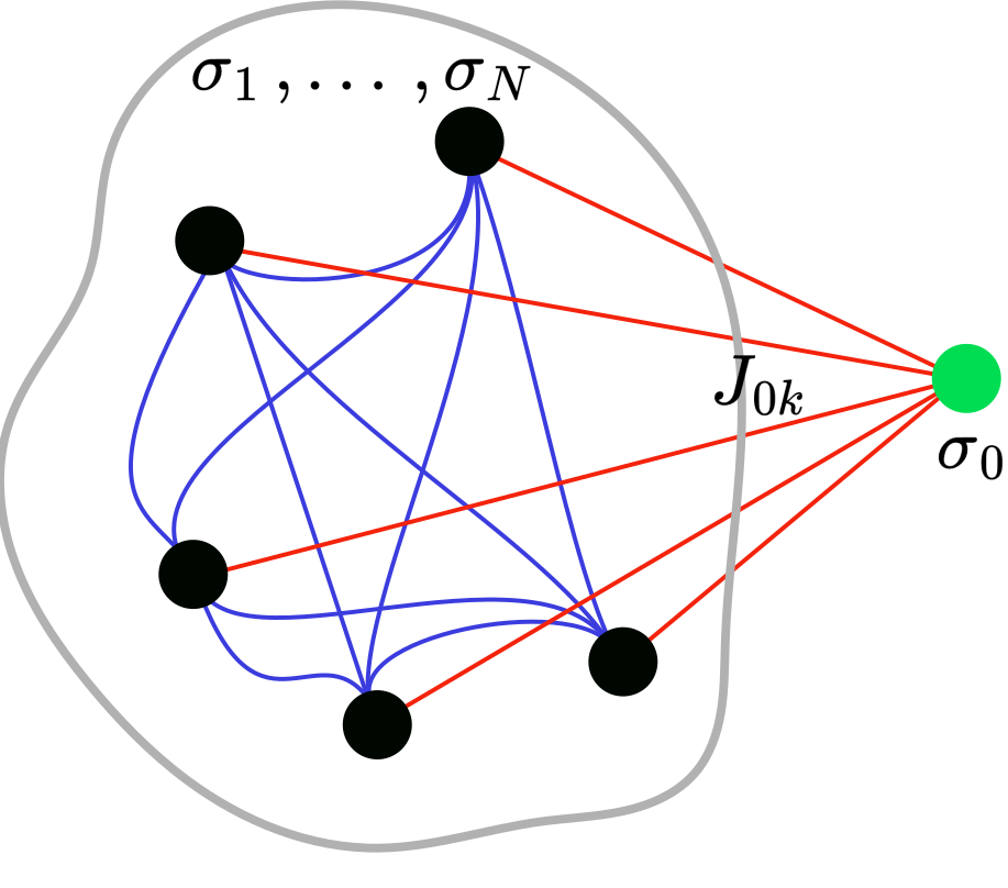
Start from an equilibrated system of $N$ spins $\sigma_1\,, \dots\,, \sigma_N$. Next imagine to add a new spin $\sigma_0$ and $N$ couplings $J_{0k} \sim \mathcal{N}(0, 1)$, $k \in [N]$ connecting $\sigma_0$ to $\sigma_1\,, \dots\,, \sigma_N$, see the figure below.

For the moment I ignore a subleading normalization issue in the couplings, and write the $(N+1)$-spin Hamiltonian as

$$H_{N+1}(\sigma,\sigma_0) = H_N(\sigma)-\sigma_0 h_0(\sigma),$$

where

$$h^{\rm cav}_0(\sigma) = \frac{1}{\sqrt{N}}\sum_{k=1}^N J_{0k}\sigma_k$$

is the instantaneous cavity field acting on the new spin. The superscript ${\rm cav}$ stresses that this field is measured in the system where the new spin is still absent. Note also that the couplings $J_{0k}$ are random variables, independent of the old system.

Using (5), the partition function of the $N+1$ spin system can be written as

$$\begin{split} Z_{N+1} &= \sum_{\sigma,\sigma_0} e^{-\beta H_N(\sigma)+\beta\sigma_0 h^{\rm cav}_0(\sigma)} \\ &= \sum_{\sigma} e^{-\beta H_N(\sigma)} 2\cosh\!\left(\beta h^{\rm cav}_0(\sigma)\right) \\ &= Z_N \left\langle 2\cosh\!\left(\beta h^{\rm cav}_0(\sigma)\right) \right\rangle_N. \end{split}$$

Here $\langle \bullet\rangle_N$ denotes the Gibbs average in the original $N$-spin system. Therefore the free-energy shift produced by the new spin is

$$\Delta F = F_{N+1}-F_N = -\frac{1}{\beta} \log \left\langle 2\cosh\!\left(\beta h^{\rm cav}_0(\sigma)\right) \right\rangle_N.$$

This equation is exact for the cavity Hamiltonian. The problem has now been reduced to understanding the distribution of the random field $h^{\rm cav}_0(\sigma)$ under the Gibbs measure of the old $N$ spin system :

$$\begin{split} P^{\rm cav}(h) &\equiv \left\langle \delta(h - h^{\rm cav}_0(\sigma)) \right\rangle_N \\ &= \frac{1}{Z_N} \sum_{\sigma} e^{-\beta H_N(\sigma)} \, \delta(h - h^{\rm cav}_0(\sigma)) \end{split}$$

This is what we call cavity field distribution.

Cavity Field Inside A State

By definition, the cavity field distribution depends on the properties of the Gibbs measure of the $N$ spin system. Let us imagine the general situation in which the Gibbs measure decomposes into pure states $\alpha$,

$$Z_N=\sum_\alpha Z_{\alpha,N}, \qquad Z_{\alpha,N}=e^{-\beta F_{\alpha,N}}\,.$$

We now condition the Gibbs measure on one such state. Inside state $\alpha$, before adding $\sigma_0$, define the cavity magnetizations

$$m_{k\to 0}^\alpha = \langle\sigma_k\rangle_{\alpha,N}^{\setminus 0},$$

and the self-overlap

$$q_\alpha = \frac{1}{N}\sum_{k=1}^N (m_{k \to 0}^\alpha)^2.$$

When $N$ is large, by the central limit theorem we should expect that the cavity field distribution is Gaussian. We therefore need to compute the first moment and the variance of the cavity field conditioned to state $\alpha$. The mean value of the cavity field in state $\alpha$ is

$$u_0^\alpha \equiv \left\langle h_0^{\rm cav}(\sigma)\right\rangle_{\alpha,N}^{\setminus 0} = \frac{1}{\sqrt{N}}\sum_{k=1}^N J_{0k}m_{k\to 0}^\alpha.$$

I will call $u_0^\alpha$ the mean cavity field, or cavity bias. This is the field to which the new spin responds once the old system is conditioned on the state $\alpha$.

Remind that, inside a pure state, connected correlations satisfy the clustering property, that is

$$\lim_{N\to\infty} \frac{1}{N^2}\sum_{i,j} \left\langle (\sigma_i-m_i^\alpha)(\sigma_j-m_j^\alpha) \right\rangle_{\alpha,N}^2 =0.$$

Using this property, we can compute the variance of the cavity field inside the state

$$\begin{split} \left\langle \left(h_0^{\rm cav}-u_0^\alpha\right)^2 \right\rangle_{\alpha,N} &= \frac{1}{N} \sum_{k,\ell} J_{0k}J_{0\ell} \left\langle (\sigma_k-m_{k \to 0}^\alpha)(\sigma_\ell-m_{\ell\to 0}^\alpha) \right\rangle_{\alpha,N} \\ &\simeq \frac{1}{N} \sum_{k=1}^N J_{0k}^2 \left[ 1-(m_{k \to 0}^\alpha)^2 \right] \\ &\to 1-q_\alpha. \end{split}$$

Therefore the cavity-field distribution inside state $\alpha$ is

$$P^{\rm cav}_\alpha(h) = \frac{1}{\sqrt{2\pi(1-q_\alpha)}} \exp\left[ -\frac{(h-u_0^\alpha)^2}{2(1-q_\alpha)} \right].$$

Equivalently,

$$h_0^{\rm cav}=u_0^\alpha+\sqrt{1-q_\alpha}\,z, \qquad z\sim\mathcal{N}(0,1),$$

Plugging this distribution into (8), and restricting to the state $\alpha$, gives

$$\begin{split} \Delta F_\alpha &= -\frac{1}{\beta} \log \int dh \, P^{\rm cav}_\alpha (h) \,$$

having denoted by $Dz$ a standard normal Gaussian measure

$$D z \equiv \frac{e^{-z^2/2}}{\sqrt{2\pi}}\, d z.$$

The first term in (18) is entropic: even inside a state the cavity field still fluctuates around its state-dependent mean. The second term is the ordinary two-state contribution of the added spin in the effective mean cavity field $u_0^\alpha$.

Cavity vs local field

It is useful to distinguish this cavity field from the local field felt by $\sigma_0$ in the $(N+1)$-spin system at equilibrium. Before adding $\sigma_0$, the field distribution in state $\alpha$ is Gaussian as in (16). After adding $\sigma_0$, configurations are reweighted by $e^{\beta h\sigma_0}$. Therefore the joint distribution of the field value $h$ and the spin $\sigma_0$ in the enlarged system is

$$P_\alpha^{\rm loc}(h,\sigma_0) = \frac{1}{\mathcal Z_\alpha} P_\alpha^{\rm cav}(h) e^{\beta h\sigma_0},$$

where

$$\mathcal Z_\alpha = \sum_{\sigma_0=\pm 1} \int dh\,P_\alpha^{\rm cav}(h)e^{\beta h\sigma_0} = e^{\frac{\beta^2}{2}(1-q_\alpha)}\,2\cosh(\beta u_0^\alpha).$$

After summing over $\sigma_0$, we obtain the local-field distribution

$$P_\alpha^{\rm loc}(h) = \frac{1}{\mathcal Z_\alpha} P_\alpha^{\rm cav}(h) 2\cosh(\beta h).$$

Notice that the local field distribution is not Gaussian! Indeed, the local field is correlated with $\sigma_0$: when $\sigma_0$ is added, it influences the spins $\sigma_1\,,\dots\,,\sigma_N$, which in turn modify the field felt by $\sigma_0$ itself. This feedback is called the Onsager reaction, discussed in the next section.

By contrast, the cavity field is measured in the system where the new spin is absent.

The Magnetization Inside A State and the TAP equations

We can now compute the magnetization of the newly added spin $\sigma_0$ in state $\alpha$ and when the $N+1$ system is equilibrated:

$$\begin{split} m^\alpha_0 &= \langle \sigma_0 \rangle_{\alpha, N+1} = \sum_{\sigma_0=\pm1}\int dh\,P_\alpha^{\rm loc}(h,\sigma_0)\,\sigma_0\\ &= \frac{\int dh\,P_\alpha^{\rm cav}(h)\,2\sinh(\beta h)}{\int dh\,P_\alpha^{\rm cav}(h)\,2\cosh(\beta h)} \\ &= \tanh(\beta u_0^\alpha). \end{split}$$

Thus the magnetization is determined by the mean cavity field $u_0^\alpha$, not by the average local field in the equilibrated $(N+1)$-spin system.

Let us now define this average local field explicitly. In the full system, the old spins have been slightly polarized by the addition of $\sigma_0$. Hence

$$H_0^\alpha \equiv$$

where now

$$m_k^\alpha=\langle\sigma_k\rangle_{\alpha,N+1}$$

denotes the magnetization in the enlarged system. This is not the same object as $u_0^\alpha$, because $u_0^\alpha$ uses the cavity magnetizations $m_{k\to0}^\alpha$ of the system in which spin $0$ is absent. Using the tilted distribution (20), the average local field can also be written as

$$\begin{split} H_0^\alpha &= \sum_{\sigma_0=\pm1}\int dh\,P_\alpha^{\rm loc}(h,\sigma_0)\,h \\ &= \frac{ \sum_{\sigma_0=\pm1} \int dh\,P_\alpha^{\rm cav}(h)e^{\beta h\sigma_0}h }{ \sum_{\sigma_0=\pm1} \int dh\,P_\alpha^{\rm cav}(h)e^{\beta h\sigma_0} } \\ &= \frac{ \sum_{\sigma_0=\pm1} e^{\beta u_0^\alpha \sigma_0} \int Dz\,e^{\beta u_0^\alpha \sqrt{1-q_\alpha}\, \sigma_0 z} \left(u_0^\alpha+\sqrt{1-q_\alpha}\,z\right) }{ \sum_{\sigma_0=\pm1} e^{\beta u_0^\alpha \sigma_0} \int Dz\,e^{\beta \sqrt{1-q_\alpha}\, \sigma_0 z} }. \end{split}$$

Using Gaussian integration by parts and equation (23), one gets

$$\begin{split} H_0^\alpha &= u_0^\alpha + \beta(1-q_\alpha) \frac{ \sum_{\sigma_0=\pm1}\sigma_0 \int Dz\,e^{\beta (u_0^\alpha+\sqrt{1-q_\alpha}\,z)\sigma_0} }{ \sum_{\sigma_0=\pm1} \int Dz\,e^{\beta (u_0^\alpha+\sqrt{1-q_\alpha}\,z)\sigma_0} } \\ &=u_0^\alpha+\beta(1-q_\alpha)m_0^\alpha. \end{split}$$

Equivalently,

$$u_0^\alpha = H_0^\alpha-\beta(1-q_\alpha)m_0^\alpha.$$

Combining (23) and (28), we obtain

$$m_0^\alpha = \tanh\!\left[ \beta\left( H_0^\alpha-\beta(1-q_\alpha)m_0^\alpha \right) \right].$$

Written for a generic spin $i$, this gives the TAP equations [Thouless, Anderson, Palmer (1977)]

$$\boxed{ m_i^\alpha = \tanh\!\left[ \beta\left( \frac{1}{\sqrt N}\sum_{j\ne i}J_{ij}m_j^\alpha - \beta(1-q_\alpha)m_i^\alpha \right) \right]. }$$

The key feature is the extra field correction

$$h_{\rm ons,i}^\alpha = -\beta(1-q_\alpha)m_i^\alpha,$$

called the Onsager reaction term. It corrects naive mean-field theory by accounting for the effect of spin $i$ back on itself through the rest of the system.

The Single-State Assumption

Replica symmetry corresponds, in this cavity language, to the assumption that there is only one relevant thermodynamic state. We can then drop the label $\alpha$ from the local magnetizations.

The cavity bias becomes

$$u_0 = \frac{1}{\sqrt{N}} \sum_{k=1}^N J_{0k}m_{k\to0}.$$

For fixed cavity magnetizations $m_{k\to0}$, this quantity fluctuates only because of the new couplings $J_{0k}$. By the central limit theorem,

$$u_0\sim\mathcal{N}(0,q), \qquad q=\frac{1}{N}\sum_{k=1}^N m_{k\to0}^2.$$

This statement concerns the mean cavity field $u_0$, not the instantaneous cavity field $h_0^{\rm cav}(\sigma)$. Inside the state, we remind the latter has the distribution

$$h_0^{\rm cav}(\sigma)=u_0+\sqrt{1-q}\,z.$$

We can now derive a self-consistent equation for the overlap. Since the new spin must be statistically equivalent to the old ones in the thermodynamic limit, its squared magnetization must reproduce the overlap $q$. Using (23),

$$m_0=\tanh(\beta u_0),$$

and averaging over the Gaussian cavity bias $u_0=\sqrt q\,z$ gives

$$\boxed{ q = \int D z\, \tanh^2\!\left(\beta\sqrt{q}\,z\right). }$$

This is the RS self-consistency equation for the overlap that can be also obtained through the replica method.

The RS Free Energy

There is one final technical point to discuss. This will in turn allow us to connect the free-energy shift to the free energy of the model.

In the true SK Hamiltonian (1) with $N+1$ spins, all couplings should be normalized by $1/\sqrt{N+1}$, while in the cavity construction above they were normalized by $1/\sqrt{N}$. This difference can be absorbed by evaluating the $(N+1)$-spin partition function at the slightly rescaled inverse temperature. The free energy shift we have computed is therefore equal to

$$\begin{split} \Delta F &= - \frac{1}{\beta} \log Z_{N+1}\left(\beta \sqrt{\frac{N+1}{N}}\right) + \frac{1}{\beta} \log Z_{N}(\beta) \\ &= - \frac{1}{\beta} \log Z_{N+1}\left(\beta \right) + \frac{1}{\beta} \log Z_{N}(\beta) - \frac{1}{2N} \frac{1}{Z_{N+1}} \frac{\partial Z_{N+1}}{\partial \beta} \end{split}$$

Taking the average over the couplings this gives the identity

$$\overline{\Delta F} = f + \frac{1}{2} \frac{\partial (\beta f)}{\partial \beta} = \frac{1}{2\beta^2} \frac{\partial}{\partial\beta} \left[ \beta^3 f(\beta) \right].$$

which connects the average free energy shift to the free energy $f(\beta)$. We can now average the state free-energy shift over the Gaussian field $h=\sqrt{q}\,z$:

$$\overline{\Delta F} = -\frac{\beta}{2}(1-q) -\frac{1}{\beta} \int D z\, \log 2\cosh\!\left(\beta\sqrt{q}\,z\right).$$

Combining (38) and (39) yields a differential equation for the RS free energy. With the high-temperature boundary condition $\beta f(\beta)\to-\log 2$ as $\beta\to0$, its solution is

$$\boxed{ f_{\mathrm{RS}}(\beta,q) = -\frac{\beta}{4}(1-q)^2 -\frac{1}{\beta} \int D z\, \log 2\cosh\!\left(\beta\sqrt{q}\,z\right). }$$

Note that the condition $\partial f_{\mathrm{RS}}/\partial q=0$ gives exactly (36). This means that the self-consistent equation for the overlap $q$ extremises $f(\beta)$:

$$\boxed{ \begin{aligned} f_{\mathrm{RS}}(\beta) &= \underset{q}{\mathrm{extr}}\, \left[ -\frac{\beta}{4}(1-q)^2 -\frac{1}{\beta} \int D z\, \log 2\cosh\!\left(\beta\sqrt{q}\,z\right) \right], \\ q &= \int D z\, \tanh^2\!\left(\beta\sqrt{q}\,z\right). \end{aligned} }$$

This is the same free energy and equation for $q$ obtained from the replica computation under the RS ansatz. The cavity derivation makes its meaning rather transparent: $q$ is the typical squared magnetization inside a single thermodynamic state, and $\sqrt{q}\,z$ is the state-dependent part of the field felt by a new spin.

At high temperature the only solution is $q=0$, and (40) reduces to

$$f_{\mathrm{RS}}(\beta,0) = -\frac{\log 2}{\beta} -\frac{\beta}{4}.$$

At low temperature a non-zero solution appears. This RS low-temperature saddle is not the full solution of the SK model: below the spin-glass transition the correct equilibrium measure requires replica-symmetry breaking. Still, the single-state cavity computation is the cleanest way of seeing where the RS equations come from and what their order parameter means.

[1] Sherrington, D. and Kirkpatrick, S., "Solvable model of a spin-glass", Physical Review Letters 35.26 (1975): 1792.

[2] Mezard, M., Parisi, G. and Virasoro, M. A., "Spin Glass Theory and Beyond", World Scientific (1987).

[3] M. Mézard, G. Parisi and M. A. Virasoro, EPL 1 77 (1986)

[4] D. J. Thouless, P. W. Anderson, and R. G. Palmer, “Solution of ‘Solvable model of a spin glass’,” Philosophical Magazine, 35(3), 593–601 (1977)