Could be worse - Random topics in statistical physics, spin glasses, optimization and average case hardness
Directed Polymers on Trees and Traveling Wavefronts
21 June 2026 | E. Malatesta
I recently came across the paper of Derrida and Spohn [Derrida and Spohn (1988)] in my research, and I found the main idea beautiful enough that I wanted to write down a self-contained post about it.
In few words, the model is a directed polymer on a disordered tree. One starts from the root of a tree and considers all directed paths of a fixed length. Each edge carries a random energy, and each path receives a Boltzmann weight depending on the total energy collected along the path. The polymer partition function is the sum of these weights over all paths.
The physics is similar in spirit to the Random Energy Model, which I discussed in two previous posts (here you can see the first and the second one). At high temperature, many paths contribute to the partition function. At low temperature, the measure condenses onto a small number of exceptionally favorable paths. In this sense, the directed polymer also has a freezing transition.
What Derrida and Spohn showed is that this freezing transition has a very elegant interpretation. The distribution of the random partition function can be encoded in a generating function, and this generating function evolves like a traveling wavefront. The low-temperature transition of the polymer is then nothing but a front-selection transition.
The goal of this post is to explain this correspondence in the discrete tree model. Derrida and Spohn also discuss a continuous-time limit, where the front equation becomes closely related to the Kolmogorov, Petrovskii, Piskunov (KPP) equation [Kolmogorov, Petrovskii, Piskunov (1937)]. That connection is useful, but here we will restrict for simplicity the discussion to the discrete model.
The model
Consider a rooted tree. Each vertex of the tree has \(K+1\) neighbors, except for the root which has \(K\) children and no parent node and for the leaves that have just one neighbor from the previous generation, see figure. We will denote the root as the ''generation'' or ''depth'' zero of the tree, the \(K\) children of the root as generation 1, the childrens of generation 1 as generation 2 and so on and so forth until generation \(n\). A directed polymer of length \(n\) is a path from the root to a node at generation \(n\)
\[ \gamma=(e_1,\dots,e_n) %= (e_{0 i_1},\dots,e_{i_{n-1} i_n}) \]Each edge \(e\) carries an independent random energy \(V_e\), sampled from a distribution \(\rho(V)\). The energy of a path is the sum over all the random energies belonging to that path
\[ E(\gamma)=\sum_{e\in\gamma}V_e. \]The partition function of the directed polymer model is
\[ Z_n(\beta) = \sum_{\gamma:|\gamma|=n} e^{-\beta E(\gamma)}. \]The total number of terms in the summation is equal to the total number of paths of length \(n\), which is equal to the total number of leaves, that is \( K^{n}\). The model naturally contains a competition between entropy and energy. At high temperature, many paths contribute to \(Z_t\). At low temperature, the partition function is dominated by a small number of exceptionally low-energy paths. The transition between these two regimes is the freezing transition.
This should remind us of the Random Energy Model: in both cases there are an exponential number of possible configurations, and the low-temperature physics is controlled by rare configurations with unusually low energy. The important difference is that the REM has independent energies, while the directed polymer model it does not. Indeed two paths that share part of their history also share the random energies on the common edges. As a result, the directed polymer keeps the same basic entropy-energy competition as the REM, but adds correlations between the energies of different paths.
The physical quantity that detects the transition is the quenched free energy density. For a finite depth \(n\) we define
\[ f_t(\beta) = - \lim_{t\to\infty} \frac{1}{\beta t} \mathbb E \left[ \log Z_t(\beta)\right], \]where \(\mathbb E\) denotes the average over the random edge energies.
The exact recursion for the partition function
The tree geometry makes the model recursive. It is convenient to write the recursion in a backward fashion, i.e. starting from the leaves and moving up toward the root. We therefore set \(t\) as the generation level measured starting from the leaves.
With a slight abuse of notation we will denote by \(Z_t\) the partition function corresponding a node at height \(t\). Thus \(t=0\) corresponds to the partition function corresponding to a leaf or an empty path, so \(Z_0=1\). Increasing \(t\) means considering larger and larger subtrees, eventually reaching the root at \(t=n\). Let
\[ Z_t^{(1)},\dots,Z_t^{(K)} \]be \(K\) independent copies of the partition function of a subtree rooted at generation \(t\).
If the first edge has energy \(V\), then every length-\((t+1)\) path is obtained by paying the first Boltzmann weight \(e^{-\beta V}\) and then choosing one of the \(K\) subtrees. Therefore
\[ \boxed{ Z_{t+1} = e^{-\beta V} \sum_{i=1}^{K} Z_t^{(i)}. } \]This is the fundamental recursion. Since \(V\) is a random variable, \(Z_{t+1}\) is a random variable as well. (6) is therefore an equation for the entire probability distribution of \(Z_t\), that we will denote as \(P_t(Z)\). We therefore have the following recursion
\[ P_{t+1}(Z) = \int \prod_{i=1}^{K} dZ^{(i)} P_t(Z^{(i)}) \int dV \, \rho(V) \, \delta\left(Z - e^{-\beta V} \sum_i Z^{(i)}\right) \]with initial condition
\[ P_0(Z) = \delta(Z-1) \,. \]The generating function
This complicated recursion (7) can be solved using a generating function. This is defined as
\[ \boxed{ G_t(x) = \mathbb E\left[ \exp\left(-e^{-\beta x}Z_t\right) \right]. } \]This is simply the Laplace transform of \(Z_t\), written with the Laplace variable
\[ s=e^{-\beta x}. \]The corresponding initial condition is
\[ \boxed{ G_0(x)=\exp(-e^{-\beta x}). } \]Let us now derive the recursion for \(G_t\). Starting from (6),
\[ Z_{t+1} = e^{-\beta V} \sum_{i=1}^{K} Z_t^{(i)}, \]we get
\[ \begin{split} G_{t+1}(x) &= \mathbb E\left[ \exp\left( -e^{-\beta x} e^{-\beta V} \sum_{i=1}^{K}Z_t^{(i)} \right) \right] \\ &= \mathbb E_V\left[ \mathbb E_{Z_t^{(1)},\dots,Z_t^{(K)}} \exp\left( -e^{-\beta(x+V)} \sum_{i=1}^{K}Z_t^{(i)} \right) \right]. \end{split} \]Since the \(Z_t^{(i)}\) are independent, the exponential factorizes:
\[ \begin{split} G_{t+1}(x) &= \mathbb E_V\left[ \prod_{i=1}^{K} \mathbb E_{Z_t^{(i)}} \exp\left( -e^{-\beta(x+V)}Z_t^{(i)} \right) \right] \\ &= \mathbb E_V\left[ G_t(x+V)^K \right]. \end{split} \]Equivalently,
\[ \boxed{ G_{t+1}(x) = \int dV\,\rho(V)\,[G_t(x+V)]^K. } \]This is the central equation of the paper of [Derrida and Spohn (1988)]. A remarkable point is that \(\beta\) has disappeared from the evolution equation. It only appears in the initial condition (11).
The generating function as a traveling wavefront
We have now reduced the polymer problem to the recursion
\[ G_{t+1}(x) = \mathbb E_V\left[G_t(x+V)^K\right]. \]The next question is: what kind of object is \(G_t(x)\)? The answer is that it has the shape of a wavefront. This section will try to hopefully convince you of that (also via a numerical solution of the recursion). Moreover we will see how that wavefront position is connected to the free energy.
The traveling wavefront
Let us introduce the variable
\[ Y_t := \frac{1}{\beta}\log Z_t. \]Substituting this into the definition of \(G_t\) gives
\[ \boxed{ G_t(x)=\mathbb E\left[\Phi_\beta(x-Y_t)\right]. } \]where we have introduced the function
\[ \Phi_\beta(u) := \exp\left(-e^{-\beta u}\right). \]The important fact is to notice that \(\Phi_\beta\) is the cumulative distribution function of a Gumbel random variable \(\xi_\beta\)
\[ \Phi_\beta(u) =\mathbb P(\xi_\beta\le u) %= \exp\left(-e^{-\beta u}\right). \]which is independent of \(Y_t\). Then, conditioning on the value of \(Y_t\), we have
\[ \begin{split} \Phi_\beta(x-Y_t) &= \mathbb P(\xi_\beta\le x-Y_t \mid Y_t) \\ &=\mathbb P(Y_t+\xi_\beta\le x \mid Y_t) \end{split} \]Taking the expectation over \(Y_t\) and using (18) we obtain the exact identity
\[ \boxed{ G_t(x) = \mathbb P(Y_t+\xi_\beta\le x). } \]Thus \(G_t\) is the cumulative distribution function of \(Y_t+\xi_\beta\). This gives the first intuition of why \(G_t\) should look like a wavefront. As \(x\) goes from \(-\infty\) to \(+\infty\), the function \(G_t(x)\) goes from \(0\) to \(1\).
Note, moreover, that the width of the Gumbel noise is of order \(1/\beta\) and is independent of \(t\). By contrast, the logarithm of the partition function grows linearly with the depth of the tree. Therefore, when \(t\) is large \(\xi_\beta\) only produces an \(O(1)\) uncertainty in the location of the wavefront \(m_t\), i.e.
\[ Y_t+\xi_\beta = Y_t+O(1) \simeq m_t \]Since we expect that \(Y_t\) concentrates when \(t\) is large, we also expect that the velocity of the wavefront is constant asymptotically. Equivalently, \(\partial_x G_t(x)\) represents the probability density of \(Y_t + \xi_\beta\). The maximum of \(\partial_x G_t(x)\), the median defined by \(G_t(m_t)=1/2\), or any other fixed level set of the wavefront all locate the same moving position of the wavefront up to an \(O(1)\) shift. Such shifts do not affect the asymptotic velocity of the wavefront.
The area swept by the wavefront and the free energy
The previous discussion says that the wavefront position \(m_t\) should be close to the typical value of
\[ \frac{1}{\beta}\log Z_t. \]Moreover as \(\lim_{t\to \infty} Y_t/ t = -f(\beta)\) we see that the free energy of the system should be connected to the velocity of the wavefront. We will here rederive this statement in a more transparent way.
For any fixed \(Z>0\), we can write the following identity
\[ \frac{1}{\beta}\log Z = \int_{-\infty}^{+\infty} \left[ e^{-e^{-\beta x}} - e^{-e^{-\beta x}Z} \right]dx. \]The proof is a one-line change of variables, and is given in the footnote.[1]
Now apply this identity to the random variable \(Z_t\) and average over the disorder. Since
\[ G_0(x)=e^{-e^{-\beta x}}, \]and
\[ G_t(x)=\mathbb E\left[e^{-e^{-\beta x}Z_t}\right], \]we obtain
\[ \boxed{ \frac{1}{\beta}\mathbb E\log Z_t = \int_{-\infty}^{+\infty} \left[ G_0(x)-G_t(x) \right]dx. } \]This identity is exact. It says that the quenched logarithm of the partition function is the area swept by the wavefront. If \(G_t\) is a wavefront that has moved a distance \(m_t\) to the right, then \(G_0-G_t\) is approximately a strip of width \(m_t\).
Suppose, more precisely, that for large \(t\)
\[ G_t(x)\simeq w(x-m_t), \]where
\[ w(-\infty)=0, \qquad w(+\infty)=1. \]If the transition region of the wavefront does not grow proportionally to \(t\), then the detailed shape of the wavefront gives only a sublinear correction to the area. Hence
\[ \int_{-\infty}^{+\infty} \left[ G_0(x)-G_t(x) \right]dx = m_t+o(t). \]Combining this with (28),
\[ \frac{1}{\beta}\mathbb E\log Z_t = m_t+o(t). \]If the wavefront moves ballistically,
\[ m_t=ct+o(t), \]then we obtain
\[ \boxed{ f(\beta) = - \lim_{t\to\infty} \frac{1}{\beta t}\mathbb E\log Z_t = -c(\beta) \,. } \]Thus the wavefront velocity is minus the physical free-energy density.
At this point the problem has become a wavefront propagation problem. The area identity tells us why the velocity matters, but it does not tell us which velocity is selected. Before computing the velocity, let us first check numerically that the recursion really behaves like a traveling wavefront.
A numerical solution of the recursive equation
We can iterate the deterministic recursion
\[ G_{t+1}(x) = \mathbb E_V\left[G_t(x+V)^K\right] \]on a grid. For Gaussian disorder,
\[ V\sim\mathcal N(0,\sigma^2), \]the recursion is
\[ G_{t+1}(x) = \int \frac{dV}{\sqrt{2\pi\sigma^2}} \exp\left(-\frac{V^2}{2\sigma^2}\right) G_t(x+V)^K. \]The code below uses Gauss-Hermite quadrature through FastGaussQuadrature.jl see additional information here.
module DP

using FastGaussQuadrature

# ------------------------------------------------------------
# Linear interpolation of G_t
#
# We impose boundary values:
# G_t(x) = 0 far to the left,
# G_t(x) = 1 far to the right.
# ------------------------------------------------------------

function interp_front(xgrid, G, y)
    if y <= xgrid[1]
        return 0.0
    elseif y >= xgrid[end]
        return 1.0
    else
        j = searchsortedlast(xgrid, y)

        x1 = xgrid[j]
        x2 = xgrid[j + 1]
        g1 = G[j]
        g2 = G[j + 1]

        return g1 + (y - x1) * (g2 - g1) / (x2 - x1)
    end
end

# ------------------------------------------------------------
# Front position m_t defined by G_t(m_t) = 1/2
# ------------------------------------------------------------

function front_position(xgrid, G; level=0.5)
    idx = findfirst(g -> g >= level, G)

    if idx === nothing
        return xgrid[end]
    elseif idx == 1
        return xgrid[1]
    else
        x1 = xgrid[idx - 1]
        x2 = xgrid[idx]
        g1 = G[idx - 1]
        g2 = G[idx]

        return x1 + (level - g1) * (x2 - x1) / (g2 - g1)
    end
end

# ------------------------------------------------------------
# One step of the recursion using Gauss-Hermite quadrature
# ------------------------------------------------------------

function one_step_quadrature!(Gnext, G, xgrid, nodes, weights; K=2, σ=1.0)
    @inbounds for i in eachindex(xgrid)
        x = xgrid[i]
        s = 0.0

        for a in eachindex(nodes)
            v = σ * nodes[a]
            y = x + v

            g = interp_front(xgrid, G, y)
            s += weights[a] * g^K
        end

        Gnext[i] = s
    end
end

# ------------------------------------------------------------
# Main function
# ------------------------------------------------------------

function simulate_wavefront(;
    β=0.7, K=2, σ=1.0,
    T=50, dx=0.1, xmin=-80.0, xmax=320.0,
    nq=100, save_times=[0, 10, 20, 30, 40, 50])


    xgrid = collect(xmin:dx:xmax)

    # Initial condition
    G = exp.(-exp.(-β .* xgrid))
    Gnext = similar(G)

    # Gauss-Hermite quadrature
    nodes, weights = gausshermite(nq; normalize=true)

    positions = zeros(T + 1)
    saved = Dict{Int, Vector{Float64}}()

    for t in 0:T
        positions[t + 1] = front_position(xgrid, G, level=0.5)

        if t in save_times
            saved[t] = copy(G)
        end

        if t < T
            one_step_quadrature!(Gnext, G, xgrid, nodes, weights; K=K, σ=σ)

            G, Gnext = Gnext, G
        end
    end

    return xgrid, positions, saved
end

end
The following script
include("polymers")
using Plots, LaTeXStrings
save_times = collect(0:2:12)
β = 0.8
T=50
xgrid, positions, saved = DP.simulate_front(β=β, T=T, save_times=save_times)
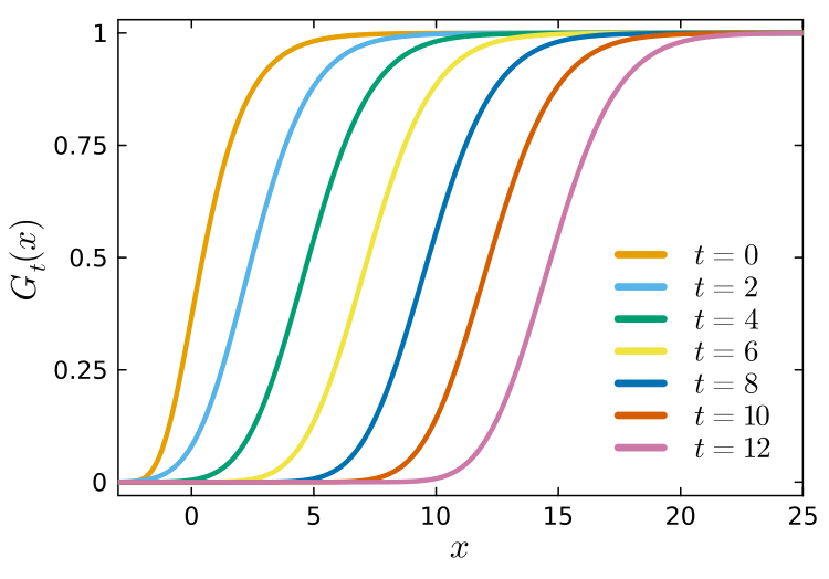
p = plot(xlabel = L"x", ylabel = L"G_t(x)", xlims = (-3.0, 25.0), label = L"t = 0")
for t in save_times
plot!(p, xgrid, saved[t], label = latexstring("\\quad t = $t"), linewidth = 3)
end
display(p)produces the plot shown below. This first plot clearly shows the appearance of a wavefront propagating to the right.
In the following script we will instead plot exactly the same wavefronts of the previous plot, but
Finally by running this script
p = plot(xlims = (-5.0, 5.0), label = L"t = 0", xlabel = L"x - m_t", ylabel = L"G_t(x)")

for t in save_times
    mt = positions[t + 1]
    plot!(p, xgrid .- mt, saved[t], label = latexstring("\\quad t = $t"), linewidth = 3)
end

display(p)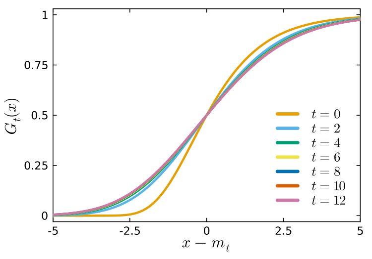
we can see that if one plots \(G_t(x)\) as a function of \(x-m_t\), with \(m_t\) defined by
\[ G_t(m_t)=\frac{1}{2}, \]the curves at different times collapse onto a common profile. This is numerical evidence for the traveling-wave form of~ (29).
Velocity selection
The area formula tells us that the free energy is minus the velocity of the front. It remains to determine which velocity the recursion selects.
As we will see, the velocity can be obtained by looking to the right leading edge of the front in the limit \(x\to \infty\), where
\[ G_t(x)\approx 1. \]Linearizing the leading edge of the wavefront
Using \(G_t=1-h_t\) in the recursion gives
\[ 1-h_{t+1}(x) = \mathbb E_V\left[(1-h_t(x+V))^K\right]. \]In the right leading edge \(h_t\ll 1\); keeping only the linear term we get
\[ \boxed{ h_{t+1}(x) = K\mathbb E_V[h_t(x+V)]. } \]with initial condition
\[ h_0(x) = 1 - G_0(x) \simeq e^{-\beta x} \]Notice that the initial profile of the right leading edge is exponential, with a steepness that depends on the inverse temperature \(\beta\). It is natural then to try an exponential profile
\[ h_t(x) = A_t \, e^{-\lambda x}, \qquad \lambda>0. \]for subsequent times also. The reason is that the linearized equation only shifts the argument of \(h_t\). A shift of an exponential profile only produces a multiplicative factor. Substituting (47) into (41) gives
\[ A_{t+1} e^{- \lambda x} = K A_t \mathbb{E}_V[e^{-\lambda V}] e^{-\lambda x} \]so
\[ A_{t} = K A_{t-1} \mathbb{E}_V[e^{-\lambda V}] = A_0 e^{t \log \left( K \mathbb{E}_V[e^{-\lambda V}]\right)} \]Because of the initial condition in equation (42) \(A_0 = 1\) so that
\[ h_t(x) = e^{-\beta x + t \log \left(K \mathbb{E}_V[e^{-\lambda V}]\right)} \]which is in the form
\[ h_t(x)= e^{-\beta(x-ct)} \]Equating the two factors, we obtain
\[ \boxed{ c(\beta) = \frac{1}{\beta} \log\left(K\mathbb E[e^{-\beta V}]\right). } \]Minimal speed and freezing
This expression of the velocity of the wavefront in equation (48) can be obtained in a simple way by computing the annealed free entropy of the model, which is reported in the footnote[2]. We have therefore to expect that (48) gives the correct prediction only in the high temperature phase. When temperature is lowered, rare disorder realizations dominate \(\mathbb E[Z_n]\).
This is reflected in the fact that equation (48) is for generic disorder distribution, not alwats a motonically decreasing function of \(\beta\), and it can possess a minimum. The existence of a minimum of \(c(\beta)\) has a simple interpretation. Increasing \(\beta\) makes the leading edge steeper, which means that the front is selecting more and more favorable low-energy paths. This initially lowers the velocity. However, very favorable paths are rare. When \(\beta\) is too large, the entropy of such paths vanishes. The velocity therefore reaches a minimum. The point where this happens is the critical point \(\beta_\star\)
\[ c'(\beta_\star)=0 \,. %\qquad %c_{\min}=c(\beta_\star). \]If \(\beta\ge\beta_\star\), the initial condition makes the wavefront too steep to make (48) satisfied at later times. It therefore moves with the minimal possible velocity. Summarizing
\[ \boxed{ c(\beta) = \begin{cases} \dfrac{1}{\beta} \log\left(K\mathbb E[e^{-\beta V}]\right), & \beta\le\beta_\star, \\[12pt] \dfrac{1}{\beta_\star} \log\left(K\mathbb E[e^{-\beta_\star V}]\right), & \beta\ge\beta_\star. \end{cases} } \]The low-temperature free energy is therefore constant for \(\beta \ge \beta_\star\). This is the frozen polymer phase.
The case of Gaussian disorder
In the case of Gaussian disorder we can see explicitly that \(c(\beta)\) (48) has a minimum. Let \(V\sim\mathcal N(0,\sigma^2). \) Then \( \mathbb E[e^{-\beta V}] = e^{\beta^2\sigma^2/2}\) and therefore
\[ \begin{split} c(\beta) &= \frac{1}{\beta} \log\left(K e^{\beta^2\sigma^2/2}\right)= \frac{\log K}{\beta} + \frac{\beta\sigma^2}{2}. \end{split} \]The critical point is determined by \(c'(\beta_\star)=0\) which gives
\[ \beta_\star = \frac{\sqrt{2\log K}}{\sigma}. \]The same critical value can also be understood from a simple entropy argument. In the footnote below, we count how many paths have a given energy density and show that the transition occurs precisely when the saddle point would move into a region with negative entropy, i.e. where the expected number of such paths is exponentially small[3].
The minimal velocity is
\[ c(\beta_\star) = \sigma\sqrt{2\log K}\,, \]so that
\[ c(\beta) = \begin{cases} \dfrac{\log K}{\beta} + \dfrac{\beta\sigma^2}{2}, & \beta\le\beta_\star, \\[12pt] \sigma\sqrt{2\log K}, & \beta\ge\beta_\star. \end{cases} \]The same code used above to iterate the wavefront recursion can also be used to compare the measured velocity with the theoretical prediction. For each time \(t\), we define the numerical velocity as \(m_t/t\), where \(m_t\) is the position of the front determined by \(G_t(m_t)=1/2\). In the Gaussian case with \(K=2\) and \(\sigma=1\), the critical inverse temperature is
\[ \beta_*=\sqrt{2\log 2}\simeq 1.177. \]The plots below show that, after a transient regime, the numerical estimate \(m_t/t\) converges toward the predicted asymptotic velocity, both in the high temperature and in the frozen phases.
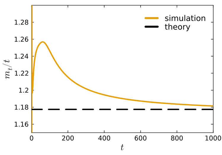
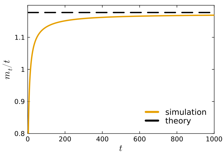
| [1] | Let us verify it. Set \[ u=e^{-\beta x}. \] Then \[ dx=-\frac{du}{\beta u}. \]As \(x\to -\infty\), one has \(u\to +\infty\). As \(x\to +\infty\), one has \(u\to 0\). Therefore \[ \begin{split} \int_{-\infty}^{+\infty} \left[ e^{-e^{-\beta x}} - e^{-e^{-\beta x}Z} \right]dx &= \frac{1}{\beta} \int_0^\infty \frac{e^{-u}-e^{-Zu}}{u}\,du. \end{split} \]Using \[ \int_0^\infty \frac{e^{-au}-e^{-bu}}{u}\,du = \log\frac{b}{a}, \]with \(a=1\) and \(b=Z\), we obtain (25). |
| [2] | The same expression for the velocity of the wavefront (48) can be obtained by computing the annealed free entropy of the model. Starting from the definition (3) we compute the disorder average \[ \mathbb E[Z_n(\beta)] = \sum_{\gamma:|\gamma|=n} \mathbb E\left[ e^{-\beta\sum_{e\in\gamma}V_e} \right]. \] For a fixed path \(\gamma\), the edge energies are independent, hence \[ \mathbb E\left[ e^{-\beta\sum_{e\in\gamma}V_e} \right] = \left( \mathbb E[e^{-\beta V}] \right)^n. \]There are \(K^n\) paths of length \(n\), so \[ \mathbb E[Z_n(\beta)] = K^n \left( \mathbb E[e^{-\beta V}] \right)^n = \left( K\mathbb E[e^{-\beta V}] \right)^n. \]Therefore \[ \begin{split} f_{\rm ann}(\beta) &= - \frac{1}{\beta n} \log \mathbb E[Z_n(\beta)] = - \frac{1}{\beta} \log\left( K\mathbb E[e^{-\beta V}] \right) \\ &= - c(\beta)\,, \end{split}\]with \(c(\beta)\) given in (48). |
| [3] | For Gaussian disorder, the energy of one fixed path of length \(t\) is Gaussian with variance \(t\sigma^2\). Therefore the probability that a given path hast energy density \(\varepsilon=E/t\) is proportional to \(\exp[-t\varepsilon^2/(2\sigma^2)]\). Since there are \(K^t\) paths, the expected number of paths \(\mathcal{N}(\varepsilon)\) with energy density close to \(\varepsilon\) is \[\mathcal{N}(\varepsilon) = e^{t \Sigma(\varepsilon)}\,, \qquad \Sigma(\varepsilon) = \log K-\varepsilon^2/(2\sigma^2)\] \(\Sigma(\varepsilon)\) being the entropy density. Then \[ Z_t(\beta) = \int d\varepsilon\, e^{t\left( \Sigma(\varepsilon)-\beta\varepsilon \right)}.\]The saddle point imposes \(\varepsilon(\beta)=-\beta\sigma^2\). This is the correct one only if \(\Sigma(\varepsilon(\beta))>0\). This gives \(\log K-\beta^2\sigma^2/2>0\), i.e. \(\beta<\sqrt{2\log K}/\sigma = \beta_\star\), the same critical point found from the wavefront velocity in (52). |
[1] B. Derrida and H. Spohn, "Polymers on disordered trees, spin glasses, and traveling waves", Journal of Statistical Physics 51, 817-840 (1988).
[2] Kolmogorov, A., Petrovskii, I. and Piskunov, N. (1937) Study of a Diffusion Equation That Is Related to the Growth of a Quality of Matter and Its Application to a Biological Problem. Moscow University Mathematics Bulletin, 1, 1-26.
[3] M. Bramson, "Convergence of solutions of the Kolmogorov equation to travelling waves", Memoirs of the American Mathematical Society 44, no. 285 (1983).